Downloading Sentinel-2 Satellite Images with Python

Sentinel-2 satellites are among the most widely used sources of Earth observation data, providing high-quality images of our planet’s surface since 2015. However, manually downloading these images can be repetitive and time-consuming. Fortunately, the OpenEO Python client allows you to download and process Sentinel-2 scenes with just a few lines of code.

What is OpenEO?

OpenEO provides standardized interfaces for seamless access to and processing of Earth observation data within the Copernicus Data Space Ecosystem (CDSE). With its versatile tools, you can effortlessly create new workflows or integrate them into existing projects.

What You’ll Learn

In this tutorial, we’ll explore how to:

• Connect to the Copernicus back-end
• Search and filter Sentinel-2 scenes
• Download and work with imagery in Python

Setting Up Your Environment

Step 1: Create a CDSE Account

First, you’ll need to set up a Copernicus Data Space Ecosystem (CDSE) account. This is the same account you use to access the Copernicus Browser for downloading scenes. You can register at https://dataspace.copernicus.eu.

Step 2: Install the OpenEO Python Client

The OpenEO Python client library is available on PyPI and can be easily installed using pip:

pip install openeo

Step 3: Install Additional Required Libraries

You’ll also need several other libraries for data manipulation, visualization, and geospatial operations:

# Install geospatial libraries
pip install rioxarray
# Install visualization library
pip install matplotlib
# Install date/time manipulation libraries
pip install pyproj python-dateutil

Connexion to the Copernicus back-end

OpenEO offers various back-ends where you can process and download satellite data. Each back-end provides different data collections and functionalities. In this tutorial, we’ll use the Copernicus back-end because it’s free to use and offers excellent access to Sentinel-2 data.

Establishing the Connection

To connect to the Copernicus Data Space Ecosystem back-end, use the following code:

import openeo
connection = openeo.connect("openeo.dataspace.copernicus.eu")
try:       
    connection = connection.authenticate_oidc(
        max_poll_time=60,  
        display=True
    )
print("✅ Authentication successful")
except Exception as e:
    print(f"❌ Authentication failed:d {e}")
    

When you run “authenticate_oidc()” for the first time, instructions will be printed with a URL you need to visit , for example: “Visit https://auth.example/?user_code=EAXD-RQXV” to authenticate. Click or copy-paste this URL into any web browser, and follow the login flow using your Copernicus Data Space Ecosystem credentials.

Once you complete the authentication in your browser, your Python script will automatically receive the necessary authentication tokens and you’ll be ready to start working with the data.

After your first authentication, OpenEO stores a refresh token on your machine, so future sessions will authenticate automatically without requiring you to visit the URL again.

Pipeline Preparation

OpenEO offers cloud computing, which means we need to first create a processing pipeline before execution. This pipeline consists of several stages:

• Filtering scenes: Select the images that match your spatial extent, temporal extent, and cloud cover criteria
• Applying masks: Remove unwanted pixels using cloud masks, shadow masks, or vegetation masks based on the Scene Classification Layer (SCL)
• Temporal reduction: Apply statistical methods (such as median, mean, or maximum) across the time dimension to create composite images from multiple acquisitions
• Band processing: Select specific spectral bands and apply any necessary transformations or calculations (such as vegetation indices) (not cover in this tutorial)
• Scale factor conversion: Convert integer to actual reflectance values
• Format conversion: Specify the output format for your results

Once the pipeline is defined, you create a batch job and launch the processing on OpenEO’s cloud infrastructure. The actual computation doesn’t happen until you explicitly start the job, allowing you to review and modify your pipeline before execution.

EO data (Collections)

In OpenEO, a back-end offers a set of collections to be processed. You can load a subset of a collection using a special process, which returns a spatial datacube. All further processing is then applied to the datacube on the back-end.

You can programmatically list the collections available on a back-end and their metadata using methods on the connection object:

collections = connection.list_collection_ids()
sentinel_collections = [c for c in collections if 'SENTINEL' in c]
print(sentinel_collections)

This collection list displays the available Sentinel collections with various processing levels applied. The processing baseline indicates the version of the processing algorithm applied to the raw data to generate the Sentinel-2 products, which particularly focuses on improving the geometric performance and radiometry of the products. In this tutorial, we’ll use SENTINEL2_L2A, which provides data from both Sentinel-2C (launched in 2024) and Sentinel-2B satellites with atmospheric corrections already applied. This collection is ideal for measuring surface reflectance and includes a Scene Classification (SCL) map that identifies clouds, snow, cloud shadows, vegetation, water, and other land cover types.

Defining your area of interest

For this tutorial, we’ll download a data cube from a field located near the French village of Arcis-sur-Aube. This location was chosen for another project aimed at studying crop health, but you can apply these methods to any area of interest.

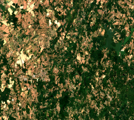
When downloading Sentinel-2 data, you need to define a bounding box large enough to capture sufficient detail in your image. If you select an area that’s too small, your image will appear overly pixelated, as shown in the example below.

It’s important to keep in mind that Sentinel-2 data has a spatial resolution ranging from 10 to 60 meters per pixel, depending on the spectral band. This means that one pixel represents a 10×10 meter area of the Earth’s surface (for the highest resolution bands).

Example calculation:

Let’s say your field is approximately 10 hectares:

• 10 hectares = 100,000 m² = 316 m × 316 m (approximately)
• With 10 m resolution: 316 m ÷ 10 m/pixel ≈ 32 pixels per side
• Total pixels for the field: 32 × 32 ≈ 1,000 pixels

So for a 10-hectare field at 10-meter resolution, you would get approximately 1,000 pixels covering your entire field. While this might seem sufficient, in practice you’ll want a larger bounding box.

Selecting the Temporal Extent

The next parameter you need to define is the temporal extent, which specifies the start date and end date of the data you want to acquire. When choosing this time range, it’s important to consider the revisit frequency of the satellites. The Sentinel-2 mission consists of two satellites (Sentinel-2B and Sentinel-2C) flying in the same orbit with a phase shift of 180°, providing a global coverage of the Earth’s land surface every 5 days.

However, there’s an important limitation: Sentinel-2 satellites are passive optical instruments, meaning they depend on sunlight to measure surface reflectance. When it’s cloudy, the satellites cannot capture usable data of the ground surface beneath the clouds. This is why it’s often necessary to:

• Select a longer time period to ensure you capture at least one cloud-free image
• Use composite methods to combine multiple images from different dates.
• Apply cloud masking using the Scene Classification Layer (SCL) to filter out cloudy pixels

For your applications, selecting a time range that spans several weeks or even months can help ensure you obtain sufficient cloud-free observations for your analysis.

from pyproj import Transformer
from datetime import datetime, timedelta
from dateutil.relativedelta import relativedelta
# coordinates of the Arcis-sur-Aube field
lon_min, lon_max = 4.15696706, 4.18226844
lat_min, lat_max = 48.58909397, 48.62135219
spatial_extent = {
        "west": lon_min, "south": lat_min,
        "east": lon_max, "north": lat_max}
#selecting temporal extent
today_date = datetime.now().date()
number_month = 3
month_3_data = today_date -timedelta(days=(number_month*30))
temporal_extent = [str(month_3_data),str(today_date)]
print(spatial_extent)
print(temporal_extent)

In our example, we’ll select a spatial extent (also called a bounding box) for a field located in France and a temporal extent of 3 months. This 3-month period should provide multiple image acquisitions, increasing our chances of obtaining cloud-free observations for analysis.

Band selection

The fourth parameter you need to specify is which spectral bands you want to download. You can check the complete list of available bands using this Python code:

connection.describe_collection("SENTINEL2_L1C")

Sentinel-2 data are acquired across 13 spectral bands in the visible and near-infrared (VNIR) and shortwave infrared (SWIR) spectrum, as shown in the table below:

Max cloud cover

The last important parameter is the maximum cloud cover, which sets the threshold for the maximum percentage of cloud coverage an image can have to be included in your results. In our example, we’ll set this to 50%, meaning only images with less than 50% cloud coverage will be downloaded.

sentinel2_cube = connection.load_collection(
    "SENTINEL2_L2A", #collection chosen
    spatial_extent=spatial_extent,
    temporal_extent=temporal_extent,
    bands=["B02", "B03", "B04","B08","B8A", "B11", "B12", "SCL"],
    max_cloud_cover=50
)

EO data

Data is represented as datacubes in openEO, which are multi-dimensional arrays with additional information about their dimensionality. Datacubes can provide a nice and tidy interface for spatiotemporal data as well as for the operations you may want to execute on them.

Data preparation

Now that we have filtered our data, we will apply some processes to prepare our image before launching the pipeline and downloading the results.

Mask clouds

The first process is to mask clouds by applying dilation to the Sen2Cor Scene Classification Layer (SCL). This dilation algorithm removes pixels in the neighborhood of clouds in a fairly aggressive manner to avoid any type of contamination. Nevertheless, some outliers can sometimes still remain.

sentinel2_cube = sentinel2_cube.process("mask_scl_dilation", data=sentinel2_cube, scl_band_name="SCL")

This algorithm uses the SCL band, which provides scene classification information including clouds, cloud shadows, snow, and other features.

Temporal reduction

The second process in our pipeline is to reduce the time dimension to create a complete image. As we discussed in the previous step, individual satellite acquisitions can be incomplete due to clouds, shadows, or other disturbances that affect the pixels in your image. To obtain a complete image with all pixels filled, we can use statistical methods to combine multiple observations over time.

median_image = sentinel2_cube.reduce_dimension(dimension="t", reducer="median")

When we reduce the time dimension ( t ) of a time series by calculating the median value, we combine all timesteps for each pixel into a single median value. This eliminates the time dimension, leaving us with a single composite image where each pixel represents the median of all cloud-free observations at that location.

The median reducer is particularly effective for creating cloud-free composites because cloud pixels with extreme brightness values don’t significantly affect the result. It selects the middle value from the time series, which is more likely to represent a clear observation and it handles missing data (masked cloud pixels) better than mean.

Scale factor conversion

The third process in our pipeline is to convert back the integer number to actual reflectance values by dividing by 10000 (or multiplying by 0.0001). Reflectance values typically range from 0 to 1.

from openeo.processes import ProcessBuilder
# define child process, use ProcessBuilder
def scale_function(x: ProcessBuilder):
    return x * 0.0001
# Convert to reflectance (simple multiplication)
print("Converting to reflectance...")
reflectance_cube= median_image.apply(scale_function)

To avoid storing long floating-point numbers and to make the files more efficient for storage and transmission, the pixel values of satellite images are converted into integer values. To preserve the dynamic range of the data, a fixed coefficient called QUANTIFICATION_VALUE (10,000 by default) is applied.

How the scaling works:

• Original reflectance value: 0.5432 (floating-point)
• Stored as integer : 5432 (= 0.5432 × 10,000)
• Converted back to reflectance: 5432 × 0.0001 = 0.5432

You can also use other scaling functions. For example, to transform satellite data into a PNG image, you can scale the values to range from 0 to 255 (the standard 8-bit range for image visualization):

def scale_function(x: ProcessBuilder):
    return x.linear_scale_range(0, 1, 0, 255)
# apply scale_function to all pixels
visual_image= reflectance_cube.apply(scale_function)

This type of scaling is useful when you want to create visualizations or export images for display purposes, rather than for scientific analysis. The ProcessBuilder allows you to define custom processing functions that can be applied to your datacube, giving you flexibility in how you transform your data.

Format conversion

The last process in our pipeline is to choose the desired output format. The save_result step is what explicitly tells OpenEO how to format your output, and it will appear as the final node in your process graph visualization. There are different formats available, but in our example we use GeoTIFF because it can store both the image data and the georeferencing information of our satellite data.

# Specify the save format 
final_result = reflectance_cube.save_result(format="GTiff")

Creating the Job and Launching the Pipeline

The result datacube object we built above describes the desired input collections, processing steps and output format. We can now just send this description to the back-end to create a batch job with the create_job method:

job_title = "Field_Observation"
job = final_result.create_job(
                title=job_title,
                description="This pipeline downloads and processes images of specific fields in France"
            )

If you’re using a Jupyter notebook, you can easily visualize the process graph by writing the job variable name in a cell:

# Display the process graph
job

In the graph below, you can check the different processes in your pipeline before launching the job. This allows you to verify that all steps are correctly configured.

The batch job, which is referenced by the returned job object, is just created at the back-end, it is not started yet. To start the job and let your Python script wait until the job has finished then download it automatically, you can use the start_and_wait method.

try:    
    result = job.start_and_wait(
                    print=lambda msg: print(f"message: [{msg}]"),
                    max_poll_interval=30, 
                    connection_retry_interval=60  
                )
    print(f"✅ Job started with ID: {job.job_id}")
except Exception as e:
    print(f"the job failed {e}")

The processing can take from a few minutes to several hours depending on:

• The size of your area of interest
• The number of timestamps in your temporal extent
• The complexity of your processing pipeline
• The current load on the back-end

Downloading the Results

Once the job is complete, you can download the results:

download_dir = "EO_data/champs1.tiff"
image = job.download_results(download_dir)
print(f"Downloaded files to {download_dir}/")

Read the image

In the last part of this article, we will read the previously downloaded image using the rioxarray library. This library is designed for working with geospatial raster data and provides convenient methods for reading, reprojecting, and manipulating georeferenced imagery.

import rioxarray
# Open the image with rioxarray
img = rioxarray.open_rasterio("EO_data/champs1.tiff")
# Reproject from WGS84 to Lambert 93
img = img.rio.reproject("EPSG:9794")

After opening the image, we reproject it to Lambert 93 (EPSG:9794), which is the official coordinate reference system for France. The Lambert 93 projection system is advantageous because it uses meters as the unit of measurement, making it easier to calculate distances and surface areas.

Visualizing the Image

You can now visualize individual bands or create RGB composites using Matplotlib and the sel method:

import matplotlib.pyplot as plt
plt.figure(figsize=(8, 8))
img.sel(band=[3, 2, 1]).plot.imshow(robust=True)
plt.title("Sentinel Image")
plt.show()

Conclusion

In this article, we explored how to download Sentinel-2 data using OpenEO in Python. We demonstrated that it’s quite easy to download and process satellite imagery with just a few lines of code. We also discussed some basics of Earth observation, including:

• Understanding Sentinel-2 collections
• Working with datacubes and multi-dimensional arrays
• Applying cloud masks and temporal reduction
• Converting scale factors to reflectance values
• Choosing appropriate output formats

What’s Next?

In the next articles, we will explore:

1. Spectral indices calculation: How to calculate different vegetation and environmental indices (NDVI, NDWI, etc.) using band reflectance values
2. Statistical methods: Preprocessing techniques to prepare data for analysis
3. Land cover classification: Creating a classification model to differentiate between:

• Bare soil
• Forests
• Agricultural fields
• Water bodies

These techniques will help you leverage satellite data for environmental monitoring, agricultural applications, and land use analysis.

References: