Building training pipelines for TikTok-like recommenders

The third lesson of the “Hands-on H&M Real-Time Personalized Recommender” open-source course.

A free course that will teach you how to build and deploy a real-time personalized recommender for H&M fashion articles using the 4-stage recommender architecture, the two-tower model design and the Hopsworks AI Lakehouse.

Lessons:

Lesson 1: Building a TikTok-like recommender

Lesson 2: Feature pipelines for TikTok-like recommenders

Lesson 3: Training pipelines for TikTok-like recommenders

Lesson 4: Deploy scalable TikTok-like recommenders

Lesson 5: Using LLMs to build TikTok-like recommenders

🔗 Learn more about the course and its outline.

Lesson 3: Training pipelines for TikTok-like recommenders

This lesson will explore the training pipeline for building and deploying effective personalized recommenders.

By the end of this lesson, you’ll learn how to:

• Master the two-tower architecture
• Create and use the Hopsworks retrieval Feature View effectively
• Train and evaluate the two-tower network and ranking model
• Upload and manage models in the Hopsworks model registry

Now, let’s dive into the “T” of the FTI Architecture by discovering how to design robust training pipelines for our real-time recommender.

💻 Explore all the lessons and the code in our freely available GitHub repository.

Table of Contents

• 1 — A short overview of the training pipeline components
• 2 — Understanding the two-tower architecture
• 3 — Building the training dataset for the two-tower network
• 4 — Training the two-tower network
• 5 — The ranking model: A short overview
• 6 — Building the ranking dataset
• 7 — Training and evaluating the ranking model
• 8 — The Hopsworks model registry
• 9 — Running the training pipeline

Enjoyed this course?

The H&M Real-Time Personalized Recommender course is part of Decoding ML’s open-source series of end-to-end AI courses.

For more similar free courses on production AI, GenAI, information retrieval, and MLOps systems, consider checking out our available courses.

1 — A short overview of the training pipeline components

Any training pipeline inputs features and labels and outputs model(s).

📚 Read more about training pipelines and their integration into ML systems [8].

In our personalized recommender uses case, the training pipeline is composed of two key parts, each serving a distinct purpose in the recommendation workflow:

1. Training the two-tower network — which is responsible for narrowing down a vast catalog of items (~millions) to a smaller set of relevant candidates (~hundreds).
2. Training the ranking model — which refines this list of candidates by assigning relevance scores to each candidate.

As a quick reminder, check out Figure 2 for how the Customer Query Model (from the two-tower architecture) and Ranking models integrate within our H&M real-time personalized recommender.

For each model, we’ll cover how to create the datasets using Hopsworks feature views, train and evaluate the models, and store them in the model registry for seamless deployment.

2 — Understanding the two-tower architecture

The two-tower architecture is the foundation of a recommender, responsible for quickly reducing a large collection of items (~ millions) to a small subset of relevant candidates (~hundreds).

While training the two-tower model, under the hood, it trains two models in parallel:

• The Query Tower, which in our case is represented by the Customer Query Encoder.
• The Candidate Tower, which in our case is represented by the Articles Encoder.

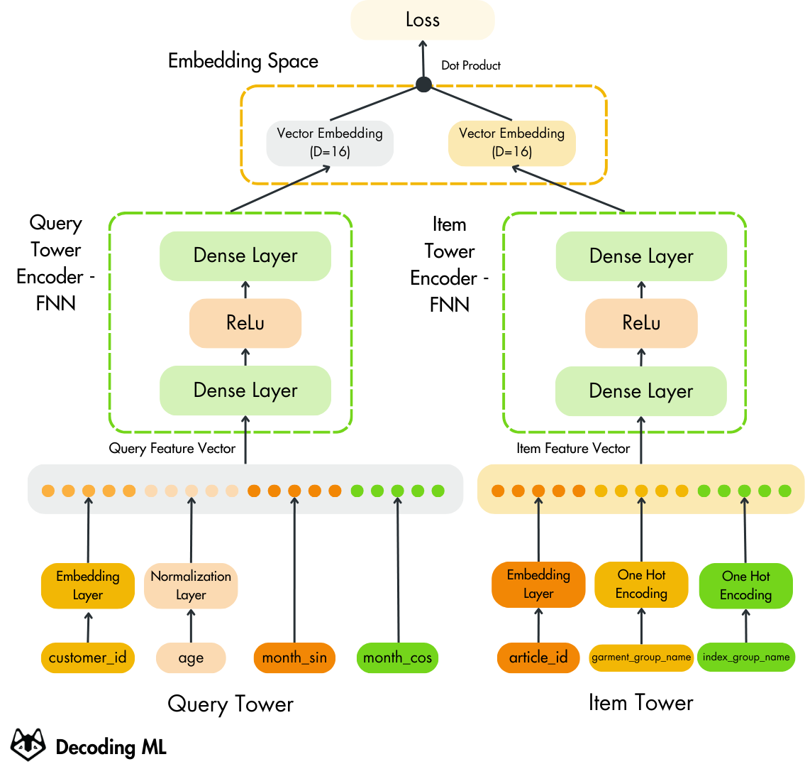
At its core, the two-tower architecture connects users and items by embedding them into a shared vector space. This allows for efficient and scalable retrieval of items for personalized recommendations.

As the name suggests, the architecture is divided into two towers:

1. The Query Tower: Encodes features about the user ( customer_id, age, month_sin, month_cos)
2. The Candidate Tower: Encodes features about the items (article_id, garment_group_name, index_group_name)

Both the Query and the Item Tower follow similar steps in embedding their respective inputs:

1. Feature encoding and fusion: In both models, features are preprocessed and combined. The customer_id and article_id are converted into dense embeddings, numeric values are normalized, and the categorical features are transformed using one-hot encoding.
2. Refinement with neural networks: A feedforward neural network with multiple dense layers refines the combined inputs into a low-dimensional embedding.

These two towers independently generate embeddings that live in the same low-dimensional space. By optimizing a similarity function (like a dot product) between these embeddings, the model learns to bring users closer to the items they are likely to interact with.

Limiting the embedding space to a low dimension is crucial to preventing overfitting. Otherwise, the model might memorize past purchases, resulting in redundant recommendations of items users already have.

We leverage the collaborative filtering paradigm by passing the customer_id and article_id as model features, which are embedded before being passed to their FNN layer.

We are pushing the network towards the content-based filtering paradigm by adding additional features to the Query Tower (age, month_sin, month_cos) and the Item Tower (garment_group_name, index_group_name). We are balancing the algorithm between the collaborative and content-based filtering paradigms depending on the number of features we add to the two-tower network (in addition to the IDs).

As an exercise, consider training the two-tower model with more features to push it to content-based filtering and see how the results change.

Having explored the two-tower architecture in depth, we continue building our model using the factory pattern.

Dig into the neural network code reflected in Figure 4 and abstracted away by the factory pattern.

query_model_factory = training.two_tower.QueryTowerFactory(dataset=dataset)
query_model = query_model_factory.build()
item_model_factory = training.two_tower.ItemTowerFactory(dataset=dataset)
item_model = item_model_factory.build()
model_factory = training.two_tower.TwoTowerFactory(dataset=dataset)
model = model_factory.build(query_model=query_model, item_model=item_model)

Read more on the two-tower architecture theory [5] or how it works with Tensorflow [2].

3 — Building the training dataset for the two-tower network

The Retrieval Feature View is the core step for preparing the training and validation datasets for the two-tower network model. Its primary role is combining user, item, and interaction data (from the feature groups) into a unified view.

We use a single dataset, the retrieval dataset, to train the query and item encoders (from the two-tower model) in parallel.

Why are Feature Views important?

Utilizing a feature view for retrieval simplifies data preparation by automating the creation of a unified dataset, ensuring:

1. Preventing training/inference skew: The features are ingested from a centralized repository for training and inference. Hence, we ensure they remain consistent between training and serving (aka inference).
2. Centralization of multiple Feature Groups: They combine features from various feature groups into a unified representation, ensuring features can easily be reused across numerous models without duplicating them, enhancing flexibility and efficiency.

For more on feature views, check out Hopsworks articles: Feature Views [3]

Defining the Feature View

To build the retrieval feature view in Hopsworks, we follow three key steps:

1. Get references to our Feature Groups: Reference the necessary feature groups from the Hopsworks feature store containing user-item interactions, user details, and item attributes.

trans_fg = fs.get_feature_group(name="transactions", version=1)
customers_fg = fs.get_feature_group(name="customers", version=1)
articles_fg = fs.get_feature_group(name="articles", version=1)

2. Select and join features: Combine relevant columns from the feature groups into a unified dataset by joining on customer_id and article_id.

selected_features = (
    trans_fg.select(["customer_id", "article_id", "t_dat", "price", "month_sin", "month_cos"])
    .join(customers_fg.select(["age", "club_member_status", "age_group"]), on="customer_id")
    .join(articles_fg.select(["garment_group_name", "index_group_name"]), on="article_id")
)

3. Create the Feature View: Use the unified dataset to create the retrieval feature view, consolidating all selected features into a reusable structure for training and inference.

feature_view = fs.get_or_create_feature_view(
    name="retrieval",
    query=selected_features,
    version=1,
)

This is our starting point for creating our training and validation datasets, as the train/test data split is performed directly on the Retrieval Feature View.

🔗 Full code here → Github

4 — Training the two-tower network

To fit our two-tower model on the Retrieval Feature View dataset, we need to define the training step, which is composed of the following:

#1. Forward Pass & Loss computation

The forward pass computes embeddings for users and items using the Query and Item Towers. The embeddings are then used to calculate the loss:

user_embeddings = self.query_model(batch)
item_embeddings = self.item_model(batch)
loss = self.task(
   user_embeddings,
   item_embeddings,
   compute_metrics=False,
)
# Handle regularization losses as well.
regularization_loss = sum(self.losses)
total_loss = loss + regularization_loss

The metrics returned by the training step are the 3 types of losses calculated earlier:

• Retrieval loss: This measures how well the model matches user embeddings to the correct item embeddings.
• Regularization loss: This prevents overfitting by adding penalties for model complexity, such as large weights. It encourages the model to generalize unseen data better.
• Total loss: The sum of the retrieval loss and regularization loss. It represents the overall objective the model is optimizing during training.

#2. Gradient computation & Weights updates

For gradient computation, we use Gradient Tape ( to record operations for automatic differentiation) and the AdamW optimizer, which has a configured learning rate and weight decay.

with tf.GradientTape() as tape:
  ...
  gradients = tape.gradient(total_loss, self.trainable_variables)
  self.optimizer.apply_gradients(zip(gradients,   self.trainable_variables))

Finally, we define the test step, where we perform a forward pass and calculate the loss metrics on unseen data from the test split of the dataset.

Our two-tower model is evaluated using the top-100 accuracy, where for each transaction in the validation set, the model generates a query embedding and retrieves the 100 closest items in the embedding space.

The top-100 accuracy reflects how often the actual purchased item appears within this subset, precisely measuring the model’s effectiveness in retrieving relevant recommendations.

🔗 Full code here → Github

Additional Evaluation Metrics

While the methods discussed earlier are standard for evaluating recommender models, others can provide more nuanced insights into performance and user relevance. Here are some key metrics to consider:

• NDCG (Normalized Discounted Cumulative Gain): A popular method for ranking that assesses both the relevance and the position of recommended items in the ranked list, giving higher importance to items placed closer to the top. Learn more about NDCG here [7].
• Other Evaluation Techniques: Metrics like Precision@K (measuring the fraction of relevant items in the top-K), Recall@K (assessing coverage of relevant items), and Mean Reciprocal Rank (MRR) (indicating how quickly the first relevant item appears) provide different insights into model performance. You can learn more about diverse metrics for recommender models here [6].

5 — The ranking model: A short overview

The ranking model refines the recommendations provided by the retrieval step by assigning a relevance score to each candidate item, ensuring that the most relevant items are presented to the user.

How It Works

1. Model input: The ranker takes the list of filtered candidate items generated by the retrieval step (from stage 2 of the 4-stage architecture).
2. Model output: It predicts the likelihood of the user interacting with each candidate, assigning a relevance score to each item based on historical transaction data.

We use the CatBoostClassifier as the ranking model because it efficiently handles categorical features, requires minimal preprocessing, and provides high accuracy with built-in support for feature importance computation.

Let’s take a quick look at how to set up our dataset, model and trainer:

X_train, X_val, y_train, y_val = feature_view_ranking.train_test_split(
    test_size=settings.RANKING_DATASET_VALIDATON_SPLIT_SIZE,
    description="Ranking training dataset",
)
model = training.ranking.RankingModelFactory.build()
trainer = training.ranking.RankingModelTrainer(
    model=model, train_dataset=(X_train, y_train), eval_dataset=(X_val, y_val))
trainer.fit()

6 — Building the ranking dataset

Creating the ranking dataset is similar to the retrieval dataset, using the same Hopsworks Feature Views functionality:

Since the CSV files only contain positive cases (where a user purchased a specific item), we must create negative samples by pairing users with items they did not buy.

As the ratio between positive and negative samples is highly imbalanced ( 1/10 ), we use the technique of Weighted Losses, which is applied through the scale_pos_weight parameter in the CatBoostClassifier constructor:

class RankingModelFactory:
    @classmethod
    def build(cls) -> CatBoostClassifier:
        return CatBoostClassifier(
            learning_rate=settings.RANKING_LEARNING_RATE,
            iterations=settings.RANKING_ITERATIONS,
            depth=10,
            scale_pos_weight=settings.RANKING_SCALE_POS_WEIGHT,
           early_stopping_rounds=settings.RANKING_EARLY_STOPPING_ROUNDS,
            use_best_model=True,
        )

Full code here → Github

7 — Training and evaluating the ranking model

Training the ranking model is relatively straightforward, thanks to CatBoost’s built-in fit and predict methods.

These are the key steps in the training process for the ranking model:

• Dataset Preparation: The datasets are converted into CatBoost’s Pool format, which efficiently handles both numerical and categorical features, ensuring the model learns effectively.

class RankingModelTrainer:
    ...
  def _initialize_dataset(self, train_dataset, eval_dataset):
          X_train, y_train = train_dataset
          X_val, y_val = eval_dataset
          cat_features = list(X_train.select_dtypes(include=["string", "object"]).columns)
          pool_train = Pool(X_train, y_train, cat_features=cat_features)
          pool_val = Pool(X_val, y_val, cat_features=cat_features)
          return pool_train, pool_val

• Training Process: The fit method is used to train the model, incorporating validation data for early stopping and performance monitoring to ensure the model generalizes well.

def fit(self):
      self._model.fit(
          self._train_dataset,
          eval_set=self._eval_dataset,
      )
      return self._model

• Model Evaluation: After training, metrics like Precision, Recall, and F1-Score are calculated to assess the model’s ability to accurately rank relevant items.

def evaluate(self, log: bool = False):
      preds = self._model.predict(self._eval_dataset)
      precision, recall, fscore, _ = precision_recall_fscore_support(
              self._y_val, preds, average="binary"
          )
      if log:
          logger.info(classification_report(self._y_val, preds))
      return {
          "precision": precision,
          "recall": recall,
          "fscore": fscore,
      }

• Compute feature importance

def get_feature_importance(self) -> dict:
    feat_to_score = {
        feature: score
        for feature, score in zip(
            self._X_train.columns,
            self._model.feature_importances_,
        )
    }
    feat_to_score = dict(
            sorted(
                feat_to_score.items(),
                key=lambda item: item[1],
                reverse=True,
            )
        )
    return feat_to_score

Full code here → Github

8 — The Hopsworks model registry

At the end of our training pipeline, we save the trained models — the two-tower model (the Query and Candidate models) and the Ranking model — in the Hopsworks Model Registry.

Storing the models in the registry is essential. This allows them to be directly deployed in the inference pipeline of your real-time personalized recommender without extra steps.

A few key points about the Hopsworks Model Registry:

• Flexible Storage: Upload your models in various formats, including Python scripts or serialized files using pickle or joblib.
• Performance Tracking: Optionally includes the model schema and metrics, allowing Hopsworks to automatically identify and retrieve the best-performing version.
• Seamless Deployment: Models stored in the registry integrate effortlessly with Hopsworks’ serving infrastructure, making them reusable across multiple pipelines.

🔗 Full documentation → Model Registry [4]

Let’s check out a top-down approach to handling a model with Hopsworks’ Model Registry by digging into the HopsworksQueryModel class.

query_model = hopsworks_integration.two_tower_serving.HopsworksQueryModel(
    model=model.query_model
)
query_model.register(
    mr=mr,
    query_df=dataset.properties["query_df"],
    emb_dim=settings.TWO_TOWER_MODEL_EMBEDDING_SIZE,
)

The HopsworksQueryModel class integrates the Hopsworks’ model registry to handle the query tower of the two-tower model.

To save our trained model in Hopsworks, we use the register() method, which can be broken down into the following steps:

1. Save the model locally:

class HopsworksQueryModel:
    ... # More code
  def register(self, mr, query_df, emb_dim) -> None:
        local_model_path = self.save_to_local()

2. Extract an input example from the DataFrame:

query_example = query_df.sample().to_dict("records")

3. Create the Tensorflow Model using the model schema, input example:

mr_query_model = mr.tensorflow.create_model(
            name="query_model",  # Name of the model
            description="Model that generates query embeddings from user and transaction features",  # Description of the model
            input_example=query_example,  # Example input for the model
            feature_view=feature_view, # Model's input feature view.
        )

Important: By attaching the feature view used to train the model, we can retrieve the exact version of the feature view the model was trained on at serving time. Thus, when the model is deployed, we guarantee that the right features will be used for inference. Eliminating one aspect of the training-inference skew.

4. Save the model to the model registry:

mr_query_model.save(local_model_path)  # Path to save the model

Once the model is registered, it can be easily retrieved at inference time together with its feature view using the Hopsworks API:

# Retrieve the 'query_model' from the Model Registry
query_model = mr.get_model(
   name="query_model",
   version=1,
)
# Retrieve the 'query_feature_view' used to train the model
query_fv = query_model.get_feature_view(init=False)

🔗 Full code here → Github

9 — Running the training pipeline

Now that we’ve covered each model in detail. Let’s take a step back to review the retrieval and ranking training pipelines:

To run the training pipelines, follow the following steps:

First, you must create an account on Hopsworks’s Serverless platform. Both making an account and running our code are free.

Next, you must run the feature pipeline to populate the Hopsworks feature groups. Afterward, you can run the training pipeline to train the models.

To run the feature and training pipelines, you have 3 options:

1. In a local Notebook or Google Colab: access instructions
2. As a Python script from the CLI, access instructions
3. GitHub Actions: access instructions

View the results in Hopsworks Serverless: Data Science → Model Registry

We recommend using GitHub Actions if you have a poor internet connection and keep getting timeout errors when loading data to Hopsworks. This happens because we push millions of items to Hopsworks.

Conclusion

This lesson taught us about the two-tower architecture, feature views, the query encoder, the candidate encoder and the ranking model.

Then, we explored how to train and evaluate these models while leveraging the features computed in the feature pipeline from Hopsworks feature views.

Lastly, we saw how to upload, version and share our trained models through the Hopsworks model registry.

In Lesson 4, we will continue with the inference pipeline, digging into implementing the 4-stage pattern and deploying it with Hopsworks and KServe.

💻 Explore all the lessons and the code in our freely available GitHub repository.

If you have questions or need clarification, feel free to ask. See you in the next session!

Enjoyed this course?

The H&M Real-Time Personalized Recommender course is part of Decoding ML’s open-source series of end-to-end AI courses.

For more similar free courses on production AI, GenAI, information retrieval, and MLOps systems, consider checking out our available courses.

Also, we provide a free weekly newsletter on AI that works in production ↓

References

Literature

[1] Decodingml. (n.d.). GitHub — decodingml/personalized-recommender-course. GitHub. https://github.com/decodingml/personalized-recommender-course

[2] Wortz, J., & Totten, J. (2023, April 19). Tensorflow deep retrieval using Two Towers architecture. Google Cloud Blog. https://cloud.google.com/blog/products/ai-machine-learning/scaling-deep-retrieval-tensorflow-two-towers-architecture

[3] Hopsworks. (n.d.-b). Overview — HopsWorks documentation. https://docs.hopsworks.ai/latest/concepts/fs/feature_view/fv_overview/

[4] Hopsworks. (n.d.). Overview — HopsWorks documentation. https://docs.hopsworks.ai/latest/concepts/mlops/registry/

[5] Hopsworks. (n.d.). What is a Two-Tower Embedding Model? — Hopsworks. https://www.hopsworks.ai/dictionary/two-tower-embedding-model

[6] 10 metrics to evaluate recommender and ranking systems. (n.d.). https://www.evidentlyai.com/ranking-metrics/evaluating-recommender-systems

[7] Normalized Discounted Cumulative Gain (NDCG) explained. (n.d.). https://www.evidentlyai.com/ranking-metrics/ndcg-metric

[8] Hopsworks. (n.d.-b). What is a Training Pipeline? — Hopsworks. https://www.hopsworks.ai/dictionary/training-pipeline

Images

If not otherwise stated, all images are created by the author.

Sponsors

Thank our sponsors for supporting our work!